All Together Now

As I revisit my generation process from top to bottom (as I do every few quarters), it might be helpful to have a flowchart or at least a process list, both for my own reference and the general welfare of the public.

1. Terrain generation, either from code or manually input (do not recommend)
2. Derive currents by a) determining major trade currents at 0 and 45 latitudes, b) extending these currents and splitting them where they hit landforms, and c) interpolating these currents via IDW to make a nice smooth surface. I also have found that d) applying a Gaussian smooth filter to the results is even nicer.
3. Assign sea surface temperature (SST) and measure the effect of the currents on that temperature: currents from the poles bringing cooler water down to the equator and vice versa.
4. Generate areas of high and low pressure
5. From the pressure map, obtain wind direction and speeds
6. Determine the effect of topography on wind
7. Apply base precipitation and use the on-shore winds to blow that moisture across the continents
8. Use the coastal current temperatures and on-shore winds to determine areas of coastal climate influence
9. Apply base temperature, then modify it according to the coastal climates
10. Lapse the temperature up mountain slopes
11. Run Koppen and Holdridge algorithms

At this point, social simulation can take over.

Wind VI: Wind Pun

Getting the wind model to work is the easy part.

Figuring out what parameters to use is the hard part.

One issue that I ran into last time is the fact that if wind starts going in the same direction from a bunch of sources, simple vector addition can add up fast.

That's because I've been treating my wind collisions as elastic collisions. There are two major kinds: elastic and inelastic. In an elastic collision, no energy is lost to heat, etc. So two (or more) winds enter a hex, one wind leaves. The following formula is used:
\[m_0 v_0 + m_1 v_1 + \cdots + m_n v_n = m_f v_f\]
This is essentially what we've been doing, in two dimensions, treating all masses as equal (even the final mass). Because I'm ignoring masses, this isn't really a physically correct description of an elastic collision.

The other option is inelastic. I think this is better, because we can think of the input winds "sticking" together into a new mass of air. This is not how fluids really mix, however, but it will be good enough. This formula is (ignoring masses again):
\[v_f = {v_0 + v_1 + \cdots + v_n \over n}\]
Which is simply the average.

So let's try a few combos of parameters. \[g\] is the ratio of decrease between each successive push, and \[z\] is the slope change (in feet) at which the wind is deflected by 45 degrees.

g=0.7, z=5000, elastic

g=0.7, z=5000, inelastic

g=0.7, z=2500, inelastic

g=0.8, z=2500, inelastic

g=0.9, z=2500, inelastic

g=0.99, z=2500, inelastic

Overall, the inelastic collision seems much more accurate. I also need to take a look at the downhill slope speed increase, which is not set for these simulations. The wind is still modulating into bands of 60 degrees, even with Gaussian blurring. Scott has trouble with straight bands, I have trouble in an additional dimension!

Also, I need to develop some better representation for topography. The heightmap is huge overkill here, but its difficult to see the effect of altitude when height is not shown at all. Something for a rainy day (of which there are many upcoming).

Wind V: Clearer Winds

As often happens, I'll publish an initial post on some subject, then add bells and whistles on to my code, then post the "finished" product with a few quips, and expect the audience to have insight into the chaos of my workflow.

So I've decided to put the wind model down on blog-paper, at least to make it clearer to myself and others. I was inspired by Here Dragons Abound, who also revisited his wind model and arrived at the same method that I did (just with better pictures)! So this post is essentially the same, just with some different words and pictures, for my own reference.

Getting the initial wind values at the coast was the easy part, really. But what to do once I have them?

Ideally, I could use some kind of iterative finite element method to solve for the flow across the surface. But that's pretty complicated and if I can find something simpler, I will.

There are a few things to keep in mind as we create this model.

• Wind slows as it drags across the ground
• Wind picks up speed when going downhill and slows uphill
• Wind is turned aside by mountains

So there are (in the most simple representation) 3 parameters that can be tuned. I'll call them $g$ for ground drag, $s$ for slope change (where $\Delta$ can represent the different in height of the hexes), and $\theta(\rho, \Delta)$ for the change in direction by a mountain (or hill, etc), where $\rho$ is the sensitivity of the wind.

Let's begin with a single wind vector.

The basic method of propagation is along the vector projection of the direction between the two hexes. I refer you to this diagram from the post on tectonics. We are interested in the $d_{\perp f}$ vector.

Projecting the vectors:

One downside of this approach is that eventually, every initial vector gets binned into one of the 6 hex directions, so the wind map becomes much more West Marches-esque, with strictly defined angles in increments of 60 degrees. But let's propagate each of these three resultants.

Next, we add the vectors (simply adding the $x$ and $y$ components) for E and B.

And of course, E and B will project onto D, and so on. But I'll ignore that for now.

So what about mountains, or other obstacles? How much is it affected? Let us assume that A represents a high mountain at 10,000 ft, and that the other hexes are 1 ft. We can then define $\theta$ in terms of $\Delta$ as:

\[\theta = {90 \exp\left(\rho\Delta\right) \over 90 + \left(\exp\left(\rho\Delta\right) - 1\right)}\]

The value $\rho={\ln(89) \over 5000}$ indicates that the wind is turned aside 45$^\circ$ at a slope of 5000 ft. So for our Mountain A, it will be 89$^\circ$. I have no idea what number will work best here. The relative direction of change is to the right in the northern hemisphere, and to the left in the southern hemisphere.

And so it continues (I haven't actually propagated A out fully).

As far as picking up speed goes, I have $s = g$ if $\Delta < 0$ else $1$. But I want to do some tweaking of this anyway (I also see a lot of stuff that I want to update/clean up, just from going through this exercise). I've been using $g = 0.946$ after my initial experiments.

So the final model for the effect of wind from Hex 0 to Hex 1 (where $h_{01}$ represents the vector from 0 to 1):

\[w_{01} = g \cdot s \cdot {w_0 \cdot h_{01} \over |h_{01}|^2} h_{01} + \angle \theta(\rho, \Delta)\]

I guess that looks kinda complicated. If you can't wow them with facts, dazzle them with bullshit.

There is also a choice to be made in the algorithm for propagating vectors. Either we can view this as an expanding frontier, where the next set of hexes to be solved is defined by where the vectors in the current frontier are pointing (projection is only ever positive for 3 hexes at most), or we can fully propagate each vector from each source (which are all coastal hexes) and then average them at the end. Right now I'm using source-propagation since its a little faster, but I'd like to take another look at frontier-propagation.

I'll save the good stuff (the actual application on the map) for another post.

Elevation XI: Uplift Revisited

One of the most important inputs to the erosion model is the tectonic uplift. I've tried a few things with this in the past, and now I'm back again for another crack at it.

The basic idea behind a hex's uplift value is its distance to convergent, transform, and divergent faults. It's difficult to compress this all into a single number, so I played around with the values until I arrived at this, where i and max_i represent the maximum distance from the C/D/T faults:

uplift = (
    0.5 * c/max_c +
    0.1 * t/max_d -
    0.4 * d/max_t + 0.399
)

So every hex will have a relative amount of uplift on a scale of 0 to 1. I do rescale this later so it goes from 0.1 to 1: no uplift means problems like sub-sea elevation terrain that I don't want to have to deal with (thanks, New Orleans).

Fault map; yellow is the highest uplift, blue is highest divergence, and white is a conjunction of all three

This number can then be fed into the erosion model to determine how much the land is rising while water is trying to eat it away. Usually, the tectonic plate wins.

So this gives us the first version of the uplift model. There are a few surprises, where I expected to see higher values, but it turns out that these are in proximity to divergent boundaries which reduce the overall number.

But this is too simple (of course). Plates don't collide like this: they ripple. There's a good approach here on one solution to this. I'll take a different tack, simply using a screening mask to to modify the values. Yet another optimization step! But this is what I will use initially, after much mucking around with different values, where $u_0$ is the initial uplift, $u_f$ is the final uplift, and $a$ is some constant.
\[u_f = \left(u_0 + {2 \sin(a u_0)\over a} + {\cos(a u_0^2) \over a}\right)^3\]

a = 50

Looks ok. Just too smooth. So we'll salt it a bit with some simplex noise:

There's still a significant problem as it relates to the overall terrain, though. There's really only one major mountain range. Everything else is at least half that value. Either 1) this is ok, and just an acceptable outcome of the inputs or 2) I can use gamma correction to modify the map.

But I'll tackle that later.

Rivers V: Muddy Waters

Now that I have the speed of rivers, I can start to figure out the balance between the deposition of sediment and the erosion of the terrain.

To reiterate, the map scale makes deposition a bit of a challenge, because the amount of sediment being picked up is enormous. This also assumes that every hex has a single drainage point.

If 1 ft of height is removed from a 347 sq.mi hex, that's nearly 275 million cubic meters of sediment that's got to go somewhere. Even if we assume that not all of it is pushed along, it's still literally tons of material.

There's a lot of studies on sediment capacities and things, but less general than I'd like - since sediment capacity and transport is something we can measure, it's not usually predicted. However, we can still draw a few conclusions.

First of all, the amount of deposited sediment is however much material is eroded away $\partial h \cdot A_h$ (where $A_h = 347$ sq.mi), plus all that's coming down the river, over the time step in question $\partial t = 2.5\cdot10^5$ yr. That's pretty straightforward.
\[Q_s = {\partial h \cdot A_h \over \partial t}\]
For a river with 70 drainage points, $Q_s = 0.369$ cu.ft/s.

We can do something similar for the amount of material that the river can hold, where $A$ is the drainage area and $S$ is the slope.
\[Q_t = k_t A^{1.5} S\]
For the river in the previous example, $Q_t = 0.836$ cu.ft/s. So the capacity is greater than that which is added to the load, and nothing happens.

$Q_s$, of course, grows as we continue down the river. So at some point it will be bigger than $Q_t$, at which point it will deposit $\partial t (Q_s - Q_t)$ cu.ft of material, or add ${\partial t \over A_h} (Q_s - Q_t)$ feet to the height of the hex. $Q_s$ is set to $Q_t$ and continues on its way.

Now, this turns out to not use velocity at all! This is alright, because knowing the velocity is still useful. There is still a lot of tweaking and testing I have to do to get this to work, and the velocity will be more helpful when determining which river routes are suitable for trade.

Elevation IX: Rivers IV: Rolling Down the River

Someone recently pointed out that my river code will probably not be satisfactory until I add deposition. I tend to agree. My code so far is merely erosion, and the models I'm modifying don't account for deposition either.

All in all, deposition is pretty important for smaller scale modelling, but it's worth considering if it could have an effect. But it turns out it's pretty complicated, and you need to know some things like the type and size of sediment each river is carrying. So I need a way to simplify the model.

However, the first thing I need to know is how fast the river is flowing. If it slows down too much, it may deposit sediment, which could end up correcting its own course.

Part of the problem I'm dealing with is again one of scale. To affect an average of 1 ft of change in a 20 mile hex, you'd need to remove (or deposit) about half a billion tons of soil. So in the real world, these things are studied on much smaller scales. Throughout this process, there are a couple of places I have to disengage from reality, if only because I'm limited in the amount of information I can provide and my sampling density.

To determine velocity, I generally need to know the discharge amount of the river, its depth and width, and the slope and roughness of the channel. None of these are easy.

There are many models relating drainage area (the only variable I really have besides slope) to the discharge amount, but they all yield numbers that are much higher than I want to use. Remember that a single hex covers 346.6 sq.mi. That's a lot of water to collect. The following equation is often offered for width in terms of drainage area (the coefficients vary across studies but are usually in this range):

\[w\textrm{ [ft]} = 13.23 \left(A\textrm{ [mi$^2$]}\right)^{0.446}\]

But this yields a channel width of 180ft for a single hex. This is probably real world realistic, but it's not what I need to use. I just don't have enough detail at this scale to say for sure if all 400 hexes are draining out at a single point on the edge of a hex. But if I just use the number of hexes (1 in this case) instead of the area, I get $w = 13$ ft. This is reasonable, even if it's not strictly accurate.

The depth of the river is another matter. In the real world, this is easy to measure, and so it's usually offered as an input rather than a result. However, I can use the same process to arrive at the following:

\[d\textrm{ [ft]} = 0.9951 \left(A\right)^{0.3012}\]

This yields a depth of a little less than a foot. That's still a fairly substantial stream - it would present a significant obstacle to trade, to say nothing of travel on foot. My small hiking experience has crossed many streams of just a few inches depth, and anything more than a foot is a noticeable, but not insurmountable, obstruction. The width to depth ratio is about 14, which is reasonable, but it has a large variation depending on very local conditions.

I considered using the Rosgen Classification, but I don't think I have enough data to make it worth it.

I need a few more geometrical parameters, the cross-sectional area, and the wetted perimeter. For now, I'll just use an ellipse to model it, although this isn't really ideal. It's not ideal because I have to use the following equations to find the perimeter:

\[\varepsilon = {\sqrt{w^2 - (2 d)^2} \over w}\]

\[P_W = w \pi \left(1 - \sum_{i=1}^\infty {(2 i)!^2\over(2^i i!)^4} {\varepsilon^{2 i}\over 2 i - 1}\right)\]

It was at this point I wondered if it's all worth it. The area is simply(er) given by:

\[A_R = {\pi w d \over 2}\]

These can be used to determine the hydraulic radius:

\[R_H = {A_R \over P_W}\]

And then the Manning Equation is used to finally determine the flow velocity:

\[v = {1 \over n}R_H^{2 \over 3}S^{1\over2}\]

Where $S = {\Delta y \over \Delta x}$, and $n$ is the Manning roughness factor, which varies depending on topography. I may use a random function to determine it in future, but for now I've set it at $n = 0.05$.

For testing, I picked a stream path at random. This once again demonstrates the scale problem. A drop of 400 ft over 20 miles is nothing. Generally speaking, walking along a slope is can be perceived at around 2.5%, which corresponds to a height change of 2640 ft. That's a lot, but of course the local terrain will be much different. All the slopes here are much less than 2%.

That yields the following profiles for slope, accumulated drainage area, and velocity in mph.

Sedimentation will be related to the river velocity; if it drops below a certain threshold, it may end changing the whole course of the river.

Current Influences

A big part of Azelor's Guide is the effect that currents have on temperatures. Generally speaking, if a warm current is near a coastline, the climate there will be warmer than it might otherwise be (Spain, for example). So this is pretty necessary for any kind of complex climate.

This should be easy (famous last words) because I already have the wind maps and the current maps. So theoretically, I just work inwards from the coasts, scaling the "degree" of influence to the wind speed. I'm not sure yet how I want to map the influence to the temperature, but that will come later.

Green - mild, blue - cold, red - hot, yellow - continental, dark yellow - continental plus

One thing I do notices is that I think the continental influence should be closer to the coast. I think I should also explore the wind model to see if I can push those winds a bit further inland. Right now, they are breaking against the elevation change, so I probably need to reduce the wind loss as it moves uphill.

First, though, I'll see how the model works when I run it on non-dummy data.

Winds II: Better Winds

Inverse distance weighting is working well. So I decided to apply it to the sea winds as well. It gives nice smooth interpolation, even if there are some places that are a bit odd. But that's ok. Nothing is perfect...yet.

Once both season (hot and cold) have been calculated, I can use the areas near the coast to define the boundary conditions for the existing land wind model. For the coastal currents only, I've categorized them as cold, hot, or mild. These aren't absolute values, just relative ones. This feeds into the precipitation model, which will be used to give better results for erosion. I'm waiting to put the finishing touches on the erosion model until I can staple these parts to it.

Elevation VIII: The Void

I'm back working on the erosion code - I think I have a better implementation, but there is an interesting problem that crops up.

I have talked before about the basin-erosion, and how it finds a way out of any place where the water might be "stuck." However, I think this mechanism is causing total collapse of the system.

Watch this gif:

It's amazing. After some cycles of building beautiful terrain, something happens. It's the Void from the Neverending Story (or Jerry's Map). Everything falls victim to the Void, swallowed by its constant advance. I haven't quite figured out why this is happening, but I have a feeling it's related to the basin-erosion code. There are a couple of places where you can see it work as intended: in one frame there will be a black gorge carved out of the mountains, and the next frame will show nice fractal patterns forming around it. However, you can also see the blackness of the Void forming around it. And once it forms...

Currents II: Getting Tide of This

I'm so, so, sorry about the pun.

That being said, the current-code is coming along. Eventually, as usual, I found a way to cheat. The only time a current should cross the ocean (at least in the initial pass) is when it's being blown by a very powerful wind, which happens around the Equator and 45$^\circ$. Outside of that, the only valid locations I'm interested in right now are those right next to the coast.

So: check to see which neighboring hexes the water can flow into. If it's valid, go there. If you hit a coast, split.

There are, of course still some issues. For one, the cellular automaton can't seem to figure out what's going on at the folds. This is a pretty common problem for me, but it's the constraint I decided to live with.

Ah, much better

Once all the coastal currents have been figured out, I'll just interpolate between everything to find out what happens in open water. A gross oversimplification, of course.

Then I'll need to figure out how that affects the on-shore winds and the moisture they carry, as well as where the hot and cold currents are (right now all the colors are red but that's just for contrast).

Currents I: Current Events

While I'm on a vector kick, I figured I'd tackle currents again. To really, truly model precipitation, I want a better model of where the hot or cold water is. I didn't actually spend that much work on it to begin with.

Most current modeling guides start off the same way. Head west along the equator, split north and south when you get to a coastline. When the current reaches about 45$^\circ$ latitude, it heads back west. If it originates from a pole, it's cold; if from the equator, it's hot. Warm and cold water meeting creates mild currents.

Theoretically that shouldn't be too hard to model. Unlike the wind model, I don't care about current strength, only direction. So I can start off with a set of vectors and propagate them out until the basics are modeled.

Keeping track of each vector is not the hard part; I just have a dictionary to store the angles. So each hex pushes water along its angle to the new target, which does the same on the next loop. The question is, what happens when I hit a coast? As mentioned before, it should split.

But, of course, this is not as simple as it seems at first. This is one of those problems where it's easy to visualize, but harder to implement in code (for me, at least). The code needs to be able to "see" the local coastline (or at least the coastal hexes) so that it can split the current in the correct directions.

For now, I've got the water moving a bit, but it won't split, and it can get trapped in a bay. The algorithm needs a way to "back out" and find an optimal path up the coast. I'm looking through a few options for classical algorithms to solve this problem (like Marching Squares or a walking algorithm).

Good

Not good

This stuff will also be useful once I extend the route finding code to the sea. It will be cheaper/easier to follow a current than to fight against it.

Wind I: Spirit of the Wind

I love what Here Dragons Abound did with wind. I want to do that, perhaps adding it to my pressure model.

Mainly, this will help with my move away from hand-drawing the rain. If I know where the wind is blowing, I can model the rain, yielding better results.

Once again, the primary source of my frustration is the sector rotation. It's hard to think in polar coordinates sometimes.

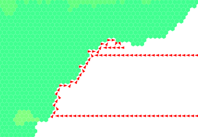
I applied a constant wind at an angle of 135$^\circ$, just for testing. The velocity is 25 knots, which is pretty high. I found a source showing a sea breeze strength of a max of 5 knots. No matter.

There are a few more rules for spreading the wind across land:

• Every time a wind is propagated, it loses 10% of its strength
• If it goes downhill, it gains some of that back depending on the slope
• If it goes uphill, it's deflected up to 90 degrees. I use a logistic function to make a nice smooth transition, using $K=90$, $P_0 = 1$, and $r={\ln(89)\over 2400}$. The rate is one of the settings I'm playing with to get a good result. The 2400 is the change in altitude where the deflection angle is 45$^\circ$. So if I want winds to make it higher up a slope, I make this number bigger.
• I talked about vector projection/rejection here, and I found that the best model for the wind is to use this to project the wind along the direction of the target hex. This "splits" the wind between the three hexes it's pointed toward the most.
• Everything gets added up using vector notation. At first I thought this propagated stuff forward too much but it seems ok after a few bugs were worked out. And I'm not using real data so that can affect things.

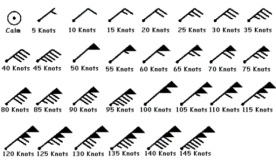
The wind barb notation shows the direction and strength of the local wind:

It's off to a good start. I'm going to think a bit more about the pressure systems so that maybe I can figure out how to integrate those into the model. There's also much tweaking to be done to get results I'm happy with.

Once that's done, I can move on to pushing moisture around.

Plenty of Faults to Go Around

Last time I said I would fractalize these puppies and see what happens. The effect is really neat - generally the fault line will take on the characteristic of its major direction, but a lot of transform faults get slipped into the mix. As a result, each tectonic line is a soup of various types of faults. This is good. It gives me that salt that I crave.

It took a little work to ensure that the fractalized lines only meet at the triple junctions, and that they generally lie the right way.

I'd also like the coastlines to line up a bit better with the geogenic faults, especially the big red ones. Anyway. I'll use this map to scale the uplifts for the terrain generation, and see if that doesn't help with the mountain ceiling problem.

Starting on Tectonics

This turned out to be harder than I thought. There's some publicly accessible information about simple vector math for fault lines, but not a ton, and of course, none of it is applicable to my particular map projection. So I had to piece together what I could. In addition, while the meeting of 4 plates at a point is technically possible, it almost never occurs, so I had to ensure while redrawing that plates only met at boundaries or triple junctions.

Thankfully, the map projection allows me to ignore the Euler vectors, which is nice, but then I have to wrap my head around correcting for all of the other transformations.

I also did all this in a really hard, really janky fashion. It's clever in that special way that avoids doing it the right way. Rather than saving the position/motion of plates at a single point, I encoded the vector in the colors of the lines themselves. This is a technique that I've been using a lot in this work, but usually in a monochromatic form. Essentially, each RGB code is a 3-channel, 256 resolution carrier for information. All I have to hardcode is those colors, write a bit of code to translate it back into motion vectors, and ta-da!

The math is a bit complex at first but eventually I figured it out to a point where it works. The important vectors are $\mathbf{d}$, which is just the relative motion of the top plate A to the bottom plate B. If this vector is pointing up, the fault is moving away from the bottom plate faster than it's moving towards it, and it's a divergent boundary (so the figure should actually show blue, not red). If $|\delta|\leq35^\circ$, the plates are moving more or less parallel to the plate (this value is arbitrary, 35 seemed good enough for what I was working with), and it's a transform boundary. I then scale the strength of divergence or convergence by the vector rejection $\mathbf{d}_{\perp\mathbf{f}}$, and if it's a transform, by the vector projection $\mathbf{d}_{\parallel\mathbf{f}}$.

There are still some zones that I need to check: R/S and I/J look odd. Then again, sometimes the combination of vectors make for interesting results. It's a neat bit of code, but nothing groundbreaking (I'll show myself out).

Next: make these lines dirty and see what happens!

Elevation IV: Fixing Endorheic Basins

About 18% of the Earth's land does not drain to the ocean. These are called endorheic basins. I need to address them for two reasons.

First of all, if water never drains all the way out to the ocean, it's hard to get up enough drainage to make any kind of appreciable river. Second, the erosion model relies on these large drainage numbers to actually modify the terrain.

So how do I deal with these? Consider the following terrain (heights shown in feet).

All the (blue) hexes bordering the center (red) hex are higher, forcing all drainage into the central hex. How do we smooth this out?

How about the average of the neighbors (10769)? This converges to a solution when applied to the overall map, although it takes a while depending on the initial inputs. The problem is that it tends to erase deep valleys - I want deep valleys! It's much too much smoothing.

The key issue is that the hex is lower than all its neighbors. I could modify one of the neighbors to be lower. This is...unsatisfactory. Unless I was making something like a moonscape. Food for thought.

There are some other features in this map that I'll talk about in a future post.

Temperature II: Interpolating Temperatures and Rain

I'm using mostly this guide on Cartographer's Guild. It's extremely helpful. One thing, though, that I've extended is the use of exact numbers for altitude, rain, temperatures, etc, rather than the use of categories. This gives me way more granular control over the result (but also introduces more problems, so YMMV).

For every climatic input, two maps are produced: summer and winter. The seasons are always reversed between hemispheres.

However, the problem (for my purposes) is that the climate undergoes a gradual change between those two points in the year. I approximate this as a sine curve, which is good enough. I've found several places where there is more than one local maximum or minimum, so even the process I'll explain here is a bit simplistic.

Let's take a hypothetical place (I'll just grab a random hex).

>>> h = choice(list(hexes))
>>> h
'98S-7W'
>>> hexes[h].temperature
{'Jul': 32, 'Jan': 57} # F
>>> hexes[h].precipitation
{'Jul': 461, 'Jan': 256} # mm

The basic equation we'll fit is:
\[y = A \sin\left(k x + \phi\right) + D, k = {2 \pi \over \lambda}\]
The amplitude is given by $A = {|t_w - t_s| \over 2}$, and the average is given by $D = {t_w + t_s \over 2}$. Since we're looking at a 12 month year, $\lambda = 12$, and so $k = {\pi \over 6}$.

The last variable, then, is $\phi$. This one is just a bit trickier. The minimum of a sine wave is at $\pi \over 4$. If we think about this in terms of 12 months, this is the 3rd month. Therefore, we need to find a value of $\phi$ such that the minimum of the sine wave matches up with the actual minimum of the data. The simple way to do this is just $\phi = 4 \textrm{ if } t_w \equiv \min(t_w,t_s) \textrm{ else } 10$.

Plugging all that in:
\[y_t(m) = {25 \over 2} \sin\left({\pi \over 6} \left(m - 4\right)\right) + 44.5^\circ\textrm{F}\]
\[y_p(m) = {205 \over 2} \sin\left({\pi \over 6} \left(m - 10\right)\right) + 358.5\textrm{ mm}\]

There are two major improvements for using this equation. First of all, I can get a much more accurate value for the total rainfall in a year (merely adding the two numbers I had gives a laughably incorrect number). The second is that (for purposes of climate) only liquid rainfall counts. That means that if the temperature in a given month is less than 32 (and here, that's the minimum, so we'd still get some freezing rain), then there is no liquid rainfall. It could still fall as snow, of course, but that has no effect on climate in Koppen or Holdridge.

With a wet winter and mild summer (not really that dry), the Koppen classification is Cfb. That's a "maritime mild winter"; think France. The Holdridge classification is perhumid subtropical wet forest, and I'm a bit skeptical of that. It'd be odd if both of those were true. I'm more inclined to believe the Koppen version, but we'll see.

To do: this assumes that, for example, the "winter" value is the lowest value. This is not necessarily the case. Perhaps the map merely shows a snapshot of January, regardless of whether January is the coldest month. So there is room for improvement. However, I took a quick look at data at various latitudes, and outside of a short transition zone around the equator, January is usually the coldest month in the northern hemisphere and the hottest in the southern, and July is the hottest in the northern and coldest in the southern. I didn't expect the transition to be as sharp as it was. Obviously, local conditions will vary. I did not do this analysis for precipitation.

Resources II: Iron Mining

Iron is a must have resource for a D&D civilization. I want to explore how iron can be found, and what other elements are found with it. I'm particularly interested in what kinds of things generally appear together. This will help me design a system for generating consistent placement of resources.

Iron has been mined for a long time. I found this article, about a Nasca ore mine, fascinating.

There are five major types of ore containing iron. There are some general trends that can help place them.

• Hematite. This is probably the most common form. It usually occurs in banded iron formations in sedimentary rock. You can also use hematite to produce various ochres, specifically in the colors of yellow, red, purple, sienna, and umber, depending on the concentration of impurities.
• Magnetite. Sometimes found in sands, but largely igneous and metamorphic rocks. It's also a good source of magnesium.
• Siderite. A poor source of iron, so I'll pretend it doesnt exist.
• Limonite. This is found in a class of soils called laterite soils. They are often found on plateaus, and contain large amounts of clay, aluminum (unknown to ancient peoples), and sometimes nickel. It's also useful for yellow ochre. More importantly, gold is often found in limonite deposits. It's generally formed in areas with alternating wet and dry seasons.
• Goethite. Commonly found in bogs, an early source of iron for the Welsh and Norse. The generation of bogs is something I'm still trying to figure out. While most of the other ores must be dug up, goethite can literally be picked up by hand out of the muck. In addition, a bog that's been picked clean generally replenishes every 50 years or so as the iron from deposits continues to coalesce. Yields brown ochre.

There is also meteoric iron, but it is so rare that any weapon made from it would certainly be an artifact and therefore priceless in any game.

Goethite and limonite are the lowest-tech and lowest-yield sources. When the limonite is worked, it actually turns into hematite. So these will be the first available in the tech system. Hematite and magnetite are harder to get and require more infrastructure and technology to extract iron from the raw ore. I need to do more thinking about what levels to assign to each of these resources. Of course, it requires additional knowledge to extract nickel and magnesium.

I'm thinking that to get a good idea of the distribution of some of these ores, I need a better system for figuring out the distribution of the different types of rock.

Resources discussed: hematite, magnetite, limonite, bog iron, clay, nickel, yellow ochre, red ochre, purple ochre, sienna ochre, umber ochre, magnesium, gold, 

Temperature I: Turn Up the Heat

I'm using the guidelines here, but I'm still looking for better ways to formulate the temperature. There is a lot of cold on my world, and a lot of hot, and not a lot of in-between. This has the potential to be pretty interesting, so I'm going to leave it for now. In such a world, control of the habitable zone would be very important.

However, most of the land is already in the southern hemisphere. I have a very deliberate north-south orientation. Many maps I see have a bias to show a vast sea to the west, no doubt tapping into cultural memories of the medieval period, or Cantre'r Gwaelod-type legends. Of course, Tolkien did us no favors with Lost Númenor.

I'd post more of these maps, but opening in Inkscape gives my computer a heart attack, since Inkscape refuses to render using the GPU. WHY? (I hear it's a planned feature...).

Summer temperatures

Black is cold, grey is warmer. Yes, it's confusing, but I map the value of the pixel to the temperature. So 0 (black) is -47 F, all the way up to ~147 (grey) for 100 F. That makes the programming a little easier.

I do work on the rough map in color to make it easier to parse in my head.

Summer temperatures

I Couldn't Think of a Pun about Potential Evapotranspiration

Hmmm. Maybe "PETs Allowed" would have worked.

Potential evapotranspiration is an important part of the Holdridge equation. Now that I have the temperature of the surface (suitably adjusted for lapse rate), I can derive the amount of water that's vaporizing from the surface. The easiest (and most inaccurate) way to figure that out is to use the Thornwaithe Equation:
\[PET = 32 \left({10 T_a \over I}\right)^\alpha,\]
where $T_a$ is the average temperature, $I$ is the heat index, and $\alpha$ is a factor derived from the heat index. All these are easily derived.

July PET map (black is lower evaporation)

Man. I really need to fix the temperature maps - right now the map thinks it's got a massive ice cap that coats nearly the entire bottom fourth of the planet. That could make for some cool Clan of the Cave Bear type adventures. But it's not what I'm looking for.

Stars and Bars

I have been thinking way too far ahead about dividing my large hexes into much smaller ones. Normally, these would be 6 miles or so - perhaps 2 mph if the mood strikes. But I have the potential to examine 1 mph...that is no simple task. Each 20 mile hex becomes 400 subhexes. How do I determine what's here? The real danger is that once that is done, I'm still not satisfied...but I should really stick to things I can accomplish right away.

Alexis has laid some excellent groundwork tying the effects of civilization to wilderness plotting. There are three posts here I'm standing on here: Groups, Features & Groups, and World Plotting. These posts deal with the generation of random subgroups of the 7 subhexes possible in a 20 mile hex. In particular, he presents a table with the odds of generating different combinations (I won't copy it here - if you want it, go there instead). A comment caught my eye, where someone considered whether this would be extendable (as I am now attempting) into larger numbers of subhexes, and hence greater detail.

I can now answer that question, a mere seven years later. This type of problem is dealt with by the combinatorics branch of mathematics, and specifically is called the Stars and Bars. The question asks, given $n$ objects, how many ways can I choose $k$ multisets? A multiset here refers to the fact that you can choose a sequence of objects that is distinct but looks the same - in Alexis's system, this is why there are only 2 distinct Type II hexes despite 7 total choices. The language here is very similar to the binomial coefficient $n\choose k$, and they are mathematically related:

\[\left(\!\!{n\choose k}\!\!\right) = {n + k - 1 \choose k} = {(n + k - 1)! \over {k! (n - 1)!}}\]

So: if we have $n = 7$ total hexes, and $k = 1$ is wilderness, then:

\[\left(\!\!{7\choose 1}\!\!\right) = 7\textrm{ total options}\]

Now that we have an abstracted model, let's return to the original equation. Fortunately, you can skip all the fancy math and just use Excel's COMBIN function. Boring (understanding the fundamentals helps with design). Here is where we encounter problems. In the 7 subhex example, the number of categories and the total number (128) of combinations are both manageable numbers. The cumulative sum is a nice, gentle slope.

Not so with 400 subhexes. There are only (let me grab my calculator) 2,582,249,878,086,908,589,655,919,172,003,011,874,329,705,792,829,223,512,830,659,356,540,647,622,016,841,194,629,645,353,280,137,831,435,903,171,972,747,493,376 total combinations. That curve is much steeper:

Hmm.

On the bright side, that pretty much guarantees that each hex will be unique (my ultimate goal), since the odds of the same layout occurring twice in 108,000 hexes (a laughably small number now) is astronomically small.

So what now?

The x-axis is tied to the infrastructure number. 7 is less than a typical infrastructure number. In the original post, the bell curve is scaled to 100. For 400 hexes, we have to compress it (assuming 100 is the max). For now, the easiest thing to do is just divide 400 by 100 and say that each point of infrastructure is worth between 1 and 4 extra hexes of not-wilderness.

These thoughts are still a bit incoherent, so I apologize. I'm trying to wrap my brain around the rule-defined system. Nobody tell Jeremy Crawford that someone is trying to use rules in D&D.