Plenty of Faults to Go Around

Last time I said I would fractalize these puppies and see what happens. The effect is really neat - generally the fault line will take on the characteristic of its major direction, but a lot of transform faults get slipped into the mix. As a result, each tectonic line is a soup of various types of faults. This is good. It gives me that salt that I crave.

It took a little work to ensure that the fractalized lines only meet at the triple junctions, and that they generally lie the right way.

I'd also like the coastlines to line up a bit better with the geogenic faults, especially the big red ones. Anyway. I'll use this map to scale the uplifts for the terrain generation, and see if that doesn't help with the mountain ceiling problem.

Starting on Tectonics

This turned out to be harder than I thought. There's some publicly accessible information about simple vector math for fault lines, but not a ton, and of course, none of it is applicable to my particular map projection. So I had to piece together what I could. In addition, while the meeting of 4 plates at a point is technically possible, it almost never occurs, so I had to ensure while redrawing that plates only met at boundaries or triple junctions.

Thankfully, the map projection allows me to ignore the Euler vectors, which is nice, but then I have to wrap my head around correcting for all of the other transformations.

I also did all this in a really hard, really janky fashion. It's clever in that special way that avoids doing it the right way. Rather than saving the position/motion of plates at a single point, I encoded the vector in the colors of the lines themselves. This is a technique that I've been using a lot in this work, but usually in a monochromatic form. Essentially, each RGB code is a 3-channel, 256 resolution carrier for information. All I have to hardcode is those colors, write a bit of code to translate it back into motion vectors, and ta-da!

The math is a bit complex at first but eventually I figured it out to a point where it works. The important vectors are $\mathbf{d}$, which is just the relative motion of the top plate A to the bottom plate B. If this vector is pointing up, the fault is moving away from the bottom plate faster than it's moving towards it, and it's a divergent boundary (so the figure should actually show blue, not red). If $|\delta|\leq35^\circ$, the plates are moving more or less parallel to the plate (this value is arbitrary, 35 seemed good enough for what I was working with), and it's a transform boundary. I then scale the strength of divergence or convergence by the vector rejection $\mathbf{d}_{\perp\mathbf{f}}$, and if it's a transform, by the vector projection $\mathbf{d}_{\parallel\mathbf{f}}$.

There are still some zones that I need to check: R/S and I/J look odd. Then again, sometimes the combination of vectors make for interesting results. It's a neat bit of code, but nothing groundbreaking (I'll show myself out).

Next: make these lines dirty and see what happens!

Elevation VII: Getting There

The growth of terrain is very slow, so I'm looking into ways to improve it. In the meantime, the algorithms as they exist seem to work pretty well, but they hit a wall. I track the highest point, with the intention of stopping the algorithm when I have a maximum height mountain, but the algorithm enters an equilibrium around 9,000 feet.

I could, of course, let the algorithm run longer, but I'd rather fix the inefficiency than let it run for a few days. The erosion code takes a few seconds to run, but the basin-fixer takes up to an hour to grind everything down.

But before I spend all that time, I think I'll work on tectonic influences a little bit more. I'd like something more than the monotonic influence along the fault. Without any internal mountain forming processes (which can be formed by buckling inside the plate or by magma plumes that break through, like Yellowstone), I need to make up for that with clever treatment of the fault line.

Resources IV: Placing Iron Ore

Once we understand some basics about the formation and location of iron ores, we can decide on an algorithm to place them.

To aid in thinking through the various prerequisites, I've begun development on charts for each one. Solid arrows mean that the condition is absolutely required. A dashed line means that it is not required, but it does improve the chance of discovery, as a modification to the chance.

Base chances will be loosely based on this chart, at least for minerals. Iron comprises about 6.3% of the crust. If I model the frequency of each ore as obeying a power law, I can use that information to figure out my base chance for each type. Hematite is the most common type by far, at least in the modern world, at 96% of all exports. That gives us the following equations, where $k$ is the power law factor, and $H$, $M = k H$, $G = k M$, and $L = k G$ represent hematite, magnetite, goethite, and limonite.
\[H + k H + k^2 H + k^3 H = H (1 + k + k^2 + k^3) = 6.3\%\]
\[{H \over H (1 + k + k^2 + k^3)} = {1 \over 1 + k + k^2 + k^3} = 96\%\]
The solution is left as an exercise to the reader. In any case, we end up with the following base chances to find our ores: $H = 6.048\%$, $M = 0.242\%$, $G = 0.00968\%$, $L = 0.000387\%$. $k$ turns out to be 4%.

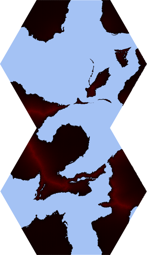
Now, these numbers are ignorant of the strictures we'd like to place. To do that, we need to know the chance that we'll actually be in an acceptable location. For example, goethite is only found in bogs, with no other strictures. The current iteration of the map has 5676 bogs, out of a possible 108132 hexes. Therefore, the chance that our dart hits a bog is only ${5676 \over 108132} = 0.052\%$. If we want to accurately distribute the goethite among them, that means that ${0.00968 \over 0.052} = 18.4\%$ of bogs will contain enough goethite to count as a resource.

Goethite bogs are concentrated in areas with heavy rainfall (the equator) and ares with poor drainage (the antarctic)

Alternatively, we could loop over the available hexes until the base chance has been reached (for goethite, that's $\sim$1045 hexes). However, that starts to increase the complexity of the placement algorithm, from $O(n)$ to something more like $O(n \cdot m^k)$. No thanks, if I can help it.

This analysis should be repeated for each resource, so that reasonably accurate numbers can be collected. Ultimately, it's enough to say that it mostly makes sense - the inherent error in these processes will serve as randomizing salt.

This set of resources is also fairly simple (goethite especially, with its single requirement). Later, I may encounter cases where there is more than one possible set of requirements. The work never ends.

Elevation VI: I Want to Be Free

Problems I can't solve tend to nag at me. Like the basin erosion. But I was reminded of a comment by Alex Schroeder a few months ago about how he lets water carve its own path out of a basin.

So I did that. It was a bit more complicated than I thought at first, since the code kept getting caught in loops. Initially, I was picking the lowest neighbors, but that was a mistake. Two hexes side by side could be each other's lowest neighbor, and they would simply trade blows until they both zeroed out. So instead, I just choose a hex randomly. This helped, at first. But I realized that the problem was that a hex is only aware of its immediate neighbors.

(I have yet to address the other part of the comment, about raising the water level until the water carves the canyon itself. My initial thought on this is to use some form of Djikstra's Algorithm to find the least-cost path to an exorheic basin, but that might clog the code even further. This generation is no joke to my poor system.)

The solution might lie in something like this, where basins are filled up working backwards from the ocean. Right now, my algorithm works by the drop model, where I start from the highest point and propagate drainage values downward. By working backwards, though, a hex always know if it ultimately drains into the sea.

This wouldn't be that hard to do. I already save the drainage directions, both in and out, for each hex. So all I have to do is follow the trail down and find out if the terminal hex is coastal or not. Still, that increases the complexity of the original algorithm. And once I know if it's part of a basin, then what?

Right now, I'm testing the following algorithm on each endorheic hex:

1. Find all hexes that drain into this one.
2. Find the lowest source hex such that at least one of its neighbors is not part of this basin (so it drains elsewhere).
3. Get the lowest valid neighbor of the source hex.
4. Follow its drainage trail until a hex is encountered that is lower than the original endorheic hex, with the added stipulation that it must be at least $\partial h$ feet lower, where $\partial h$ is the number of hexes between the two so far. So if there are 4 hexes between the endorheic hex and the river source, and 6 hexes between the source and the new low, then $\partial h = 10$.
5. Adjust the altitude along the new path so that there is a constant slope from the endorheic hex to the new low hex.

Once this is completed for all endorheics, the new drainage network can be found and checked to see if we've hit our target number. If not, repeat. There are still a couple of edge cases to handle: if it hits another basin, if it hits a flat area, etc. The biggest problem with this is that it's very very slow. I loathe to even estimate the Big O complexity.

Fairly good

Not so good

That being said, a good solution is desirable regardless of time. So I may just have to deal with it. I don't have to run it every single iteration of the erosion mountain growth. That will require some more experimentation. In additional, I'll run erosion after it as well, so the spidery lines above might get washed out.

Elevation V: I Want to See Mountains Again!

I've put the endorheic code aside for now. It's making everything much too smooth.

Instead, I'm trying to fit the original tectonic faults back into the system. The map from the endorheic basins post was one such map.

The keys here are fiddling with the original maps and with the uplift map, which determines how much the land is affected by the tectonic collisions.

For one thing, I need to add more plates, now that the system is a little more extendable. I don't really want to mess with the coastline, but right now the terrain is really boring on a couple of these continents.

The other thing is adding a factor to push the coastal hexes down towards the sea. Otherwise, hexes with no appreciable drainage (islands) end up being the limiting factor (the erosion cycles run until one of the hexes maxes out at 25,599 feet).

I can also start with some white noise as the initial map (instead of designing them by hand) and see where things lead. Remember that erosion is partially a function of rainfall, and I painted those maps using the original height maps. I should probably paint them based on the uplift map (which is based on the fault lines). Here Dragons Abound did something very similar, although there are enough slight differences that it's worth tackling from scratch for me.

Since I don't have a way (yet) to model the force of collision, I will simulate folds by assigning an uplift scaling factor $u$ based on the distance to the fault line $f$ and distance to the coast $d$.
\[u = \left(\exp\left(-f \over 500\right)\cdot\left(1 + 0.1\cos\left({2\pi \over 100} f\right)\right) + 0.1\right)\cdot\left(0.9999\left(1-\exp\left({-d \over 20}\right)\right) + 0.0001\right)\]
Simple.

That yields this as the initial uplift:

So the mountains should grow out of this after enough cycles. Man, I really should add more tectonic plates. There's an entire continent there (top/bottom left, I really should assign some temporary names) with very little tectonic activity.

When I was writing this post, I intended to come back and show the result of that map. But I tried something else instead. I added a little bit of Perlin noise to the uplift map. Now this could be something interesting.

Can't tell that much difference. But it's nice to "salt" things a little.

Elevation IV: Fixing Endorheic Basins

About 18% of the Earth's land does not drain to the ocean. These are called endorheic basins. I need to address them for two reasons.

First of all, if water never drains all the way out to the ocean, it's hard to get up enough drainage to make any kind of appreciable river. Second, the erosion model relies on these large drainage numbers to actually modify the terrain.

So how do I deal with these? Consider the following terrain (heights shown in feet).

All the (blue) hexes bordering the center (red) hex are higher, forcing all drainage into the central hex. How do we smooth this out?

How about the average of the neighbors (10769)? This converges to a solution when applied to the overall map, although it takes a while depending on the initial inputs. The problem is that it tends to erase deep valleys - I want deep valleys! It's much too much smoothing.

The key issue is that the hex is lower than all its neighbors. I could modify one of the neighbors to be lower. This is...unsatisfactory. Unless I was making something like a moonscape. Food for thought.

There are some other features in this map that I'll talk about in a future post.

Demoland Infrastructure Map

I swore I wouldn't start mapping 1-mile hexes. There's still so much to be done, but this article got me thinking again about applying changes to the landscape based on infrastructure.

Essentially, I use this process to randomize a hex into two types of meta-terrain: wilderness and not-wilderness. Eventually, I'd like to further abstract this system, but for now, it makes pretty-ish maps.

• I've set the maximum displayable infrastructure as 100, but I think that should be changed to 400 (1 per subhex).
• Road placement would be really cool to see on this.
• How big is that river, really?
• The city labels are a little hard to see.

A Lasting Impression

Maybe you've seen this fascinating article floating around. The recent heat fluctuations in Wales have unveiled long-buried remains of hillforts and towns.

"The buried ramparts of Cross Oak Hillfort, Talybont-on-Usk, showing as crop marks in Powys." Credit: RCAHMW

This made me think about the effects of civilization on terrain. I'm working on vegetation cover right now, and if the conditions are right, forest will cover much of the surface of the planet. Obviously, this is affected by the current population, but it's also affected by those who have lived there before. I'm definitely going to be thinking about this more when I tackle the procedural history problem. Today, in real life, we have grassland plains and meadows caused by the deforestation of ancient peoples, where there should be woodland. This should be apparent from the ebb and flow of the terrain.

Consider how your ancient civilizations shaped the land under the unsuspecting feet of your more modern cities.

Roads I: Original Pathfinder

No, not that pathfinder. To be honest, I've never played it.

I'm talking about a real pathfinder.

Where do the roads go? How can I get from Point A to Point B most effectively?

I won't try to give an indepth explanation of how the algorithm I've chosen (A*) works, since others can do that much better. I'll just explain how I implemented it.

def a_star(start, end):
  def g(current):
        z = zip(closed_list, closed_list[1:] + [current])
        return sum(travel(i, j) for i, j in z)
    def h(current):
        return(distance(hexes[current].c, hexes[end].c) / 86.6)
    def f(current):
        return g(current) + h(current)
    open_list = list(hexes[start].neighbors)
    closed_list = [start]
    came_from = {sorted(open_list, key = lambda h: f(h))[0]: start}
    while open_list:
        s = sorted(open_list, key = lambda h: f(h))[0]
        open_list.remove(s)
        closed_list.append(s)
        if s == end:
            break
        for t in hexes[s].neighbors:
            if t not in closed_list:
                if t not in open_list or g(t) < h(t):
                    open_list.append(t)
                came_from.update({t: s})
    path = [end]
    while path[-1:][0] != start:
        path.append(came_from[path[-1:][0]])
    return path[::-1]

Basically, we find the path that minimizes the cost of travel. I've made some custom adjustments to the travel heuristic here. The only modifications so far are for height - I need to work on more specific terrain later. For now, moving up or down 400 feet costs an extra day of travel. If you're moving into or through an area that's above 8000 feet, it costs an extra day for each 1000 more feet you ascend (due to oxygen requirements - 8000 feet is the general baseline I've found, but I'm not a climber, and I'd like some better data to use here).

Here, it is quite obvious that even those constraints are enough to create an interesting pathway. Rather than take the "shortest" path (a straight line), our caravan is compelled to ascend into the foothills, and follow the crests of the mountain chain, until at last a suitable pass is found.

This took about two hours to implement - much better than I was expecting. I think the next steps are to figure out the effects of terrain, and to save the cumulative road score (how many paths are found through this hex), which can affect the desirability index. High traffic roads are good places to start up a village and leech off the resulting trade.

One thing I don't know how to do yet is sea travel. This is an important one, but there are a few problems.

1. I don't save sea hexes as terrain; I leave them blank to save file size
2. Sea travel is highly dependent on winds and currents, which I have, but not in a format that is good for cellular automata

There are ways around these problems, but I have to pick them out of my brain first. Right now they're floating around nebulously and I can't see them very clearly.

Temperature II: Interpolating Temperatures and Rain

I'm using mostly this guide on Cartographer's Guild. It's extremely helpful. One thing, though, that I've extended is the use of exact numbers for altitude, rain, temperatures, etc, rather than the use of categories. This gives me way more granular control over the result (but also introduces more problems, so YMMV).

For every climatic input, two maps are produced: summer and winter. The seasons are always reversed between hemispheres.

However, the problem (for my purposes) is that the climate undergoes a gradual change between those two points in the year. I approximate this as a sine curve, which is good enough. I've found several places where there is more than one local maximum or minimum, so even the process I'll explain here is a bit simplistic.

Let's take a hypothetical place (I'll just grab a random hex).

>>> h = choice(list(hexes))
>>> h
'98S-7W'
>>> hexes[h].temperature
{'Jul': 32, 'Jan': 57} # F
>>> hexes[h].precipitation
{'Jul': 461, 'Jan': 256} # mm

The basic equation we'll fit is:
\[y = A \sin\left(k x + \phi\right) + D, k = {2 \pi \over \lambda}\]
The amplitude is given by $A = {|t_w - t_s| \over 2}$, and the average is given by $D = {t_w + t_s \over 2}$. Since we're looking at a 12 month year, $\lambda = 12$, and so $k = {\pi \over 6}$.

The last variable, then, is $\phi$. This one is just a bit trickier. The minimum of a sine wave is at $\pi \over 4$. If we think about this in terms of 12 months, this is the 3rd month. Therefore, we need to find a value of $\phi$ such that the minimum of the sine wave matches up with the actual minimum of the data. The simple way to do this is just $\phi = 4 \textrm{ if } t_w \equiv \min(t_w,t_s) \textrm{ else } 10$.

Plugging all that in:
\[y_t(m) = {25 \over 2} \sin\left({\pi \over 6} \left(m - 4\right)\right) + 44.5^\circ\textrm{F}\]
\[y_p(m) = {205 \over 2} \sin\left({\pi \over 6} \left(m - 10\right)\right) + 358.5\textrm{ mm}\]

There are two major improvements for using this equation. First of all, I can get a much more accurate value for the total rainfall in a year (merely adding the two numbers I had gives a laughably incorrect number). The second is that (for purposes of climate) only liquid rainfall counts. That means that if the temperature in a given month is less than 32 (and here, that's the minimum, so we'd still get some freezing rain), then there is no liquid rainfall. It could still fall as snow, of course, but that has no effect on climate in Koppen or Holdridge.

With a wet winter and mild summer (not really that dry), the Koppen classification is Cfb. That's a "maritime mild winter"; think France. The Holdridge classification is perhumid subtropical wet forest, and I'm a bit skeptical of that. It'd be odd if both of those were true. I'm more inclined to believe the Koppen version, but we'll see.

To do: this assumes that, for example, the "winter" value is the lowest value. This is not necessarily the case. Perhaps the map merely shows a snapshot of January, regardless of whether January is the coldest month. So there is room for improvement. However, I took a quick look at data at various latitudes, and outside of a short transition zone around the equator, January is usually the coldest month in the northern hemisphere and the hottest in the southern, and July is the hottest in the northern and coldest in the southern. I didn't expect the transition to be as sharp as it was. Obviously, local conditions will vary. I did not do this analysis for precipitation.

Rivers III: Eroding the Coast

As I've continued to tweak the erosion system, I want to start working on how this erosion affects the coast. This is one of those projects that's big enough in scale that I don't even want to start; however, it's the perfect type of job to do when I'm hitting mental roadblocks elsewhere.

The first thing I did was identify all hexes lower than 50 feet. Next, I go through them and manually modify the coastline to include those hexes; if they're that low, the sea has encroached, or they've hit the water table.

A quick note: the height of the water table often means that lakes can be at very high altitude. There are some very clever ways to approximate this, but I'll leave those for another day.

Another note: while my system can deposit within my already-defined coasts (mostly seen as tectonic uplift), there is no mechanism to add new hexes to those in the land set. That might be a problem but again, not one I want to solve right now.

I'll repeat this process a few times, since I'm redoing the precipitation maps almost once a week now. Just cannot get them perfect. But the pursuit of perfection is itself a goal.

Resources III: Copper Mining

Copper is not quite as easy to get as iron. Unlike bog iron, copper is only available once mining itself is available as a local technology. There are many modern sources of copper, but I'll focus on three as my main ones.

• Chalcopyrite. Found in porphyry copper deposits, which I am going to associate mostly with volcanic areas. It also shows up in coal seams.
• Malachite. This is possibly the oldest source of copper, as the Egyptians were using malachite ores very early in their history. It is also used as a blue pigment.
• Azurite. The best use for this is not as copper ore, but as green pigment. It's almost always found alongside malachite.

The next step once you have copper is to add tin. That of course makes bronze, and you can make fairly good weapons, at least until you figure out how to make iron and then steel.

Resources discussed: chalopyrite, malachite, azurite, green pigment (malachite), blue pigment (malachite), gold, coal, azure