Resources XXII: Reserves

I will be going through material sources in an effort to quantify which areas would be most suitable for population generation. To do this I'll rely on the concept of reserves.

On the Higher Path blog [subscription needed], Alexis calls out reserves as:

So let's use the word Reserves to describe wealth as it occurs in the wilderness, and resources to describe wealth as that which the civilised parts of the kingdom actively exploit.

I'll use it in a slightly different way: the level of unexploited resource in the wilderness which may be exploited. Not all wells are equally deep, for instance.

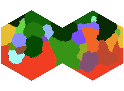
Let us consider the noble auroch. This animal occurs in the following Koppen climates: Aw; As; Am; Csa; Csb; Csc; Cwa; Cwb; Cwc; Cfa; Cfb; Cfc; Dfa; Dfb. As a large mammal, we may also assume it needs at least 1 point of water drainage in a hex to survive (probably a low estimate). This yields the following distribution:

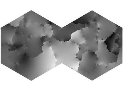
Nothing interesting so far. Let's apply some Perlin noise.

Now, aurochs are not found in every place where they might possibly be. For the sake of illustration, let's do 50% (cattle are pretty ubiquitous, I'd expect this to be on the high side for a reserve).

We are left with a number between 0 and 1 detailing the relative level of abundance of the wild reserve of aurochs. What that level is can then be derived separately and scaled. For example, wild cattle generally form herds of about 10 animals, with some instances of up to 184 head/3400 hectares. This is less than a reference per hex: about 0.3 ref/20hex. Obviously, once these herds are domesticated, their size will increase, so the exact relationship between the raw reserve and its resource equivalent will need to be defined.

On the other hand, I could simply tie the 0-1 relative abundance to the maximum developed reference density, which for this resource is 733 ref/20hex (assuming 100% utilization which is obviously a false assumption). Much to think about.

The advantage of using Perlin noise is the fact that it is reproducible given the same inputs: if these are defined for each commodity, then the reserves sort themselves out.

The Juvenis Adventure

For the last few weeks, I've been lucky enough to be a player in Alexis' reboot campaign, the Juvenis Adventure.

The experience has been quite something even in early stages. Play-by-post is a tricky mistress, and even more so when the players stretch across many time zones. Alexis' game is hard work at times, but it's different from every campaign I've ever been in.

My fresh-off-the-boat elven fighter was thrown more or less immediately into a fight which far outclassed me. The party had last left off fighting demon toads and attempting to close a gate to Hell itself. Oh sure, I've been in (and run) similar scenarios before; so what was so different about this one?

The difference crystallized in a single moment: we attempted to swing an icy gate shut and a demon teleported right next to me to prevent us from moving it. My Level 1 fighter had no magical weapons, an overly cautious demeanor towards combat, and no health to speak of. I knew this demon could kill me and cast my soul into Hell, probably all in the same turn.

And there's the difference: I had to decide to stand and fight (and protect my friends) or to run and maybe save myself. I felt real fear in the pit of my stomach - my character had no backstory to save, no valuables to protect - a coldness in my heart weighing my options. I had to overcome an actual emotion, to swallow my pride and put my body in the breach.

That is something you won't find in any other game.

Koppen and Holdridge

The last step in climate is to apply the Koppen or Holdridge mappings, based on the local temperature and precipitation properties.

I'm not at all convinced that Holdridge is working for me. But I like to keep it around just in case.

Holdridge key

Holdridge

Overall, Koppen seems more intuitively correct.

Koppen key

Koppen

A nice mix of types of terrain. For some reason I feel like Koppen is easier to work with. Maybe it's the palette. Using all this data, I assign a terrain value (such as forest or savanna). This lets me make a map which is more human friendly.

Terrain

There's a lot of savanna here, as it turns out. I can live with that.

I think the next thing I'll dive into is individual resource research. I want to start gaming at some point in the next ten years, so it's necessary to get some actual stuff a party could use (as well as the historical simulation for background). That'll be a project in itself.

Temperature VI: PET

I have previously addressed potential evapotranspiration here, so I don't really need to address it again beyond a few minor updates.

January

July

Temperature V: Big Picture

To find the temperature, I created functions that more or less followed the guidelines from this post. The best way I found was to have slightly different functions for each category.

'normal': lambda x: -42.5 * (x / 90) ** 2 + 25 if x >=0 else -20 * (-x / 90) ** 2 + 25,
'hot': lambda x: -42.5 * (x / 90) ** 2 + 25 if x >=0 else -20 * (-x / 90) ** 4 + 25,
'cold': lambda x: -42.5 * (x / 90) ** 1.5 + 25 if x >=0 else -20 * (-x / 90) ** 1 + 25,
'cont': lambda x: -63 * (x / 90) ** 2 + 25 if x >=0 else -56.5 * (-x / 90) ** 2 + 25,
'cont+': lambda x: -63 * (x / 90) ** 2 + 25 if x >=0 else -20 * (-x / 90) ** 2 + 25

Then I just flip it around (reverse the latitude) in the opposite season. The common theme remains: the important thing is that this code exists and can be easily applied.

The next step is a small blur to smooth out the transitions, and then I lapse the temperature up based on height (-3.5 F per 1000 ft).

January

January

Looks reasonable to me, although I probably should fiddle with the map colors so that the hot and cold areas pop a bit more.

Temperature IV: Coastal Influence

Coastal and continental influences help make the temperature distribution more interesting.

With winds and current temperatures well in hand, should be easy enough to find these areas where cold and hot temperatures (here defined simply where the current is colder or warmer than the default temperature) are distributed near the coast.

In these plots, blue and red represent cold and hot influences. Yellow represents continental influence (large landmasses) and dark yellow is "continental plus."

January

July

...Quite a lot of cold current influence, to be perfectly honest. I was expecting more of a mix. This tells me I might need to do some work on my current temperature algorithm.

For now, however, this part of the code works. Garbage in, garbage out, so I will need to return to the "in garbage" at some point soon.

The other explanation is that the large landmass across the equator prevents true recirculation of the warmest waters. The poles, which generate the cold currents, are relatively unchallenged. So perhaps there is an explanation here where the code remains ok.

Rain II

Now we can begin to get closer to the meat of climate.

I begin with the base precipitation value at the coasts: \[P_h = p_0 \cdot \left(\exp\left(\frac{-\left(\ell - s\right)^2}{\sigma^2}\right) + \\ \frac{1}{2} \cdot \exp\left(\frac{-\left(\ell - 45 s\right)^2}{\sigma^2}\right) + \frac{1}{2} \cdot \exp\left(\frac{-\left(\ell + 45 - s\right)^2}{\sigma^2}\right)\right) \frac{(90 - \ell)(90 + \ell)}{90^2}\], where $p_0$ is the max precipitation value (127 mm/mo), $\ell$ is the latitude, $s$ is a seasonal parameter (15 in summer, -15 in winter), and $\sigma=19.5$.

Wet vs dry coasts (summer)

Throw in a box blur (n=3, radius=2) and baby, you got a stew goin'.

January

July

So far I like these results more than the first time around. Onward!

Wind VIII: Over the Land to Skye

Once we have established the wind pattern over the sea, we can determine the effect that the topography has on those winds.

First, I get a list of all winds blowing on or near the coasts. For each of those, I take the projected vector of the wind onto each neighboring hex. If the angle of the projected vector is $<90^\circ$, I know that it's at least in the right direction to catch a bit of that wind.

From there, I determine $dh$, which is the difference between the heights of the two hexes, source and target. If $dh$ is downhill ($dh<0$), there's no change. Otherwise, the turnaside angle $\theta$ is calculated as \[\theta = \frac{90 \exp\left(r \cdot \mathit{dh}\right)}{90 + \left(\exp\left(r \cdot \mathit{dh}\right) - 1\right)}\], where $r=2\log(89)/5000$ is calculated such that the wind will be totally turned aside $90^\circ$ when the slope is 5000 ft or more.

This is one of those areas that I've still not managed to tweak completely to my satisfaction, but it will be good enough to use for precipitation.

Angle of wind vectors (not speed) in summer

Wind VII

I'm looking over my old code and wondering what on earth I actually did to make this work.

Or whether it worked at all.

Allegedly, I used a curl function to boil the pressure down into a wind value (wind rotates around pressure centers, this makes sense). But I had gotten that initial pressure from a hand-drawn map on GIMP, and that's what I'm trying to get away from in this latest attack.

I tried to fiddle with getting the gradient but the implementation of a discrete gradient on a hex grid was somewhat problematic. However, this value may be useful later on in determining the length of the wind vector - winds on a steep pressure gradient will naturally be stronger.

The angle is another matter. This is where I really thought the gradient would help (and maybe it would on a different grid or even map layout). I ended up doing something much simpler: "walk" around the edge of the major pressure cells, correcting for direction based on the Coriolis effect, then (predictably) use IDW to fill in the rest of the map.

a quarter million objects has more of an effect on performance than you might think

For now, I am not box-blurring these values, so the transitions are still a little choppy. My plan is to apply the effect of the topography on the wind vectors and then smooth it out, so that everything lines up more nicer.

Pressure II

Update from here.

This time around, since I'm avoiding all manual input as much as possible, I can programmatically generate the pressure bands, at least a rough approximation of them.

The first step is pretty simple, I just apply the rules from this post to hexes which meet the correct criteria.

Then to smooth it out, I apply a box blur with a radius of 10 hexes to the pressure values (which are scaled between -1 and 1). I do this 3 times to approximate a Gaussian blur. Since I'm doing this on a hex grid, I haven't yet figured out any of the clever optimization tricks that are available for this approximation on a square grid.

January (winter in the north)

July (summer in the north)

For my next trick, I will try to avoid memory leaks while calculating wind flow.

Currents VI: The Hand of Franklin

With the current code updated, I tackled water temperature and icecap formation.

Warm water from one region will move to a colder region, and vice versa. Where does this happen?

First, I assign a temperature to all water cells based on season and latitude $\ell$. Compared to some of my other functions, it's a little boring: \[T_\ell = \begin{cases}-50 & \text{if $\ell < 0$} \\ -57 & \text{otherwise}\end{cases}\cdot\left(\frac{\ell}{90}\right)^{\begin{cases}4 & \text{if $\ell<0$} \\ 2 & \text{otherwise}\end{cases}}\] This is different from my calculation of air temperature.

Once that is done, I "push" that water around for 80 hexes - an arbitrary number, but whatever. Then I take the average of all the water that has entered a new cell, and there we have the new temperature.

light blue: water that is colder than expected

My next move is to check where the water temperature is below freezing, to see how the ice caps look. I have to do a bit of cleaning here because otherwise I get a whole bunch of unconnected floating bergs - which ain't terribly realistic. But after convincing the water of what I think it should be really doing instead, I get a nice permanent ice cap (dark blue), with a seasonal glaciation shown in light blue.

North Pole

South Pole

The shapes aren't mindblowingly realistic but they'll do for my purposes. Of particular interest are potential harbors which become walled off by icebergs during the cold season, as well as any effects the caps might have on navigational routes: it might be quicker to tempt the poles, but depending on the level of sailing technology it might be wise to steer well clear of even the temporary caps.

Next, I'll revisit wind generation, then return to sea temperature to see where the cold water is affecting coastal climate.

All Together Now

As I revisit my generation process from top to bottom (as I do every few quarters), it might be helpful to have a flowchart or at least a process list, both for my own reference and the general welfare of the public.

1. Terrain generation, either from code or manually input (do not recommend)
2. Derive currents by a) determining major trade currents at 0 and 45 latitudes, b) extending these currents and splitting them where they hit landforms, and c) interpolating these currents via IDW to make a nice smooth surface. I also have found that d) applying a Gaussian smooth filter to the results is even nicer.
3. Assign sea surface temperature (SST) and measure the effect of the currents on that temperature: currents from the poles bringing cooler water down to the equator and vice versa.
4. Generate areas of high and low pressure
5. From the pressure map, obtain wind direction and speeds
6. Determine the effect of topography on wind
7. Apply base precipitation and use the on-shore winds to blow that moisture across the continents
8. Use the coastal current temperatures and on-shore winds to determine areas of coastal climate influence
9. Apply base temperature, then modify it according to the coastal climates
10. Lapse the temperature up mountain slopes
11. Run Koppen and Holdridge algorithms

At this point, social simulation can take over.

Currents V: Refresher

Try to avoid SVGs with a quarter million linked objects, if you can.

In the meantime, the currents are looking nice when applied to the generated terrain surface.

I begin with a handful of hexes in the ocean, on the coasts where the trade winds are blowing more or less perpendicularly into the ocean. I then propagate this current forward (curving around the map folds). When the current reaches an opposite coast, it curves back around.

The next step is to fill in all the gaps using IDW (with nearest neighbor distance $k=20$ and exponent $n=2$), which I've used quite commonly in the past for many applications. It's a really useful little algorithm. This generates a smooth fill.

Lastly, I apply a Gaussian filter to smooth out the sharp bits even more.

This has proven more than adequate for my needs, especially concerning the influence of cold and warm coastal currents, as well as trade and migration routes further down the line. The possibilities present themselves endlessly.

Elevation XVII: Lift Up Your Heads

I've been working on the topography generator for quite some time now. I think it's time to put a pin in it. There's still so much to be done, but I need to take a break.

It's looking much better than it was. The endorheic algorithm, which helps basins find their way to the sea, is by far the most inefficient/slow part of the code, and so I think future iterations may try to address that.

GIF of elevation+erosion algorithm at work

This is a good opportunity to start working back through all the rest of the climate generation code to bring life to this map (and by extension, any other generated topography). There is a lot of clean-up to do.

Elevation XVI: Clean Your Plate

I'm still not ready to do full tectonic movement simulations.

However, I think I can get some mileage out of using plates themselves to generate a better uplift map. The code for this is pretty simple, some general flood-fill algorithms along the fault lines:

In this model, each hex is only affected by the faults it actually borders:

This gives us some smooth transitions and some stark differences - which I feel effectively captures the action of subducting and overlapping plate faults.

In reality, the difference between ocean and land is not a unimodal curve. Earth differs in this regard because it has uniquely defined oceans in the first place.

However, no one is interested in fitting a curve to this specific shape. Until now.

This consists of a piecewise curve as:
\[
h_1(x) = 55 \exp\left(-\frac{x}{0.65}\right)\textrm{ if }x >= 0
\] \[
h_2(x) = 55 \exp\left(\frac{x}{0.15}\right)\textrm{ if }x < 0
\] \[
h_3(x) = 15 \exp\left(-\left(\frac{x + 4.6}{1.5\sqrt{2}}\right)^2\right)\textrm{ if }x < 0
\]
Where the full cumulative distribution is given by \[H(x) = \int_{-11}^x h_1(n) + h_2(n) + h_3(n)\textrm{ d}n\]

This is in units of 1000 km, which is not what I want. However, if I scale both the inputs and outputs to $[0,1]$, I get a non-linear I/O curve similar to a gamma correction.

Hm.

Doesn't look quite how I wanted it. Lets do a simulation run.

Starting to see some of those shapes: but the distribution is not great. Most of the mountain chains are reasonably distributed except for the big pile in the middle.

I'll continue to work on this. I'm getting closer to what I want.

Elevation XV: From Square One

I wanted to take a break from prehistory stuff while I read up on hunter-gatherer sociology. I decided to revisit terrain generation.

My current terrain was created by drawing continents I liked, loosely matching them with tectonics, generating uplift values from that, then performing hydraulic erosion until I liked it. I'm still not ready to move into tectonic simulation, but I wanted some landforms that more closely mimicked the plates I'd drawn. I also took the opportunity to clean up the hydraulic erosion code.

It turns out, perhaps predictably, that the tectonic input map is perhaps the most important variable of all.

Fault map, showing convergent influence in red (with transform in green and divergent in blue)

I experimented with a variety of drop-off functions (Gaussians, other exponentials) to find a good way to find the closest fault (or most influential fault, by strength) to a given hex. This took a really long time, because I had to iterate over ~2000 fault hexes for each of the ~250000 world hexes. Some Poisson sampling helped, but even then, my uplift map ends up with circular ripples.

Uplift map: the Poisson disks are particularly obvious along the convergent equatorial fault

Where the uplift map is too patterned, the landforms tend to be also. So I tried adding in various kinds of warped and ridged noise to try and mix up those forms. One big problem with using noise of any kind is that it looks much too uniform at all scales. A quick look at Earth's coastline reveals a variety of types of "noisy" coastline, some smooth, some rough. So any kind of realistic noise function will need to approximate this variety. The hydraulic erosion discussed below can help with this. However, I still think more work is needed to obtain a better fault/uplift map from the input tectonics. One on-going issue is that the basic tectonic distribution persists from the time when I did most of my work by direct sketching. Maybe next week I'll work a bit on a generated (or at least computed) fault map to add more variety.

There are four basic processes which can alter the altitude of a hex: d$u$, the uplift of the plate; d$e$, the removal through erosion; d$s$, the deposition of transported sediment (from eroded material); d$c$, coastal erosion.

Although I had used a simplified version of this model before, I hadn't considered some practical limits:

• A hex will stop eroding once it is completely "ground down," that is, its height is equal to the height of the hex to which it drains. At this point, water no longer flows. Hexes under sea-level do not erode with the same mechanism. For now, I've turned it off, but a possible alternative is a constant rate of erosion. As always, erosion rate is determined by how many hexes drain into the target.
• On the other end, once a hex has been completely filled with sediment, it won't accept any more drainage. This one is a bit more complicated: I compare the height of the hex to the height of all other options that the source hex could use. Once the sediment makes the hex no longer the lowest of all the source's neighbors, drainage will instead flow into the new target. So it might not necessarily reach the height of the source.
• Coastal erosion stops once the hex has been eroded under sea level. The erosion rate is faster the more sides are exposed to the ocean. I think it might be interesting to continue to transport and deposit that sediment elsewhere, but that would require the current model to run every iteration.

The coastlines look pretty good but the overall landforms indicate I need to do more work with tectonics and uplift